M. Ducceschi, C. Webb and G. Fratoni

Efficient synthesis of large room impulse responses in the modal domain

This article introduces a linear modal framework for the identification and synthesis of room impulse responses (RIRs) over large frequency bands. A sub-band implementation of the PolyMAX algorithm is employed for parameter extraction, followed by time-domain reconstruction via second-order oscillator banks.

A sub-band implementation of the PolyMAX algorithm, orginally developed in the context of experimental modal analysis in structural mechanics, may be applied to extract the modal parameters of the target system.

The PolyMAX algorithm proceeds in two stages: first, the poles of the transfer function are obtained via a linear-in-parameters least-square optimisation along with the computation of the poles of the transfer function via the eigenvalue of the companion matrix. Importantly, the model order is increased to build a stabilisation diagram, from which stable poles may be identified, and spurious "mathematical" poles are excluded. After collecting poles, a second least-square optimisation is performed to

Mathematical Formulation of Modal Identification

Let \( H(z) \in \mathbb{C} \) denote the discrete-time frequency response of a measured system, for scaling time constat \( T \). The system is modelled as a rational transfer function:

\[ H(z) \;=\; \frac{B(z)}{A(z)} \;=\; \frac{b_0 + b_1 z + \cdots + b_{p}z^p}{a_0 + a_1 z + \cdots + a_{p}z^p}\, \]

where \( A \) and \( B \) are polynomials of order \( p \).

Given discrete frequency response data from a measured RIR, the transfer function above is evaluated on a number \(N\) of discrete frequency bins, such that: \[ \hat H_k := \hat H\left(e^{j\omega_k T}\right), \quad k = 0,1,...,N-1, \]

where the “hat” notation denotes a measured response. The coefficients of \( A(z) \) and \( B(z) \) can be determined by solving a linear least-squares problem. Specifically, approximating (FRF model) with the measured response gives:

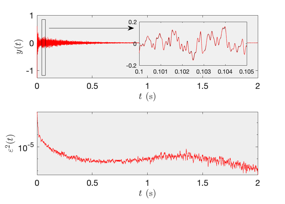
\[ \epsilon_k := B_k - A_k\,\hat H_k \approx 0, \]

for each frequency sample \( \omega_k \) in the dataset. In matrix form:

\[ \boldsymbol{\epsilon} = [\mathbf{X}, \mathbf{Y}]\begin{bmatrix}\boldsymbol{\beta}\\\boldsymbol{\alpha}\end{bmatrix}, \]

where \( \mathbf{X}, \mathbf{Y} \in \mathbb{C}^{N \times (p+1)} \), with:

\[ (\mathbf{X})_{k,:} = \left[1,e^{j\omega_k T},\ldots,e^{j p \omega_k T}\right], \] \[ (\mathbf{Y})_{k,:} = -\hat H_k \cdot (\mathbf{X})_{k,:}, \] \[ \boldsymbol{\beta} = [b_0,b_1,\ldots,b_p]^\intercal, \quad \boldsymbol{\alpha} = [a_0,a_1,\ldots,a_p]^\intercal. \]

Least-square minimisation

A linear-in-parameters least-squares minimisation is readily available for the norm of \( \boldsymbol{\epsilon} \). The optimisation problem is defined as:

\[ \min_{\boldsymbol{\beta}, \boldsymbol{\alpha} \in \mathbb{R}^{p+1}} \frac{1}{2}\|\boldsymbol{\epsilon}\|^2_2\,. \]

First, note that:

\[ \|\boldsymbol{\epsilon}\|^2_2 = [\boldsymbol{\beta}^\intercal, \boldsymbol{\alpha}^\intercal] \begin{bmatrix}\mathbf{R} & \mathbf{S} \\ \mathbf{S}^\intercal & \mathbf{T}\end{bmatrix} \begin{bmatrix}\boldsymbol{\beta}\\\boldsymbol{\alpha}\end{bmatrix}, \]

with \( \mathbf{R} := \operatorname{Re}(\mathbf{X}^\dagger\mathbf{X}) \), \( \mathbf{S} := \operatorname{Re}(\mathbf{X}^\dagger\mathbf{Y}) \), \( \mathbf{T} := \operatorname{Re}(\mathbf{Y}^\dagger\mathbf{Y}) \). The symbol \( \dagger \) denotes the Hermitian transpose.

Setting gradients to zero gives the normal equations:

\[ \begin{aligned} \mathbf{R}\boldsymbol{\beta} &= -\mathbf{S}\boldsymbol{\alpha}, \\ \mathbf{T}\boldsymbol{\alpha} &= -\mathbf{S}^\intercal \boldsymbol{\beta}. \end{aligned} \]

Using the first in the second:

\[ \left(\mathbf{T} - \mathbf{S}^\intercal \mathbf{R}^{-1}\mathbf{S} \right)\boldsymbol{\alpha} := \mathbf{M}\boldsymbol{\alpha} = 0. \]

To avoid the trivial solution, set \( a_p = 1 \) and solve:

\[ \mathbf{A}\boldsymbol{\alpha}_{0:p-1} = \mathbf{b} \]

with \( \mathbf{A} := \mathbf{M}_{0:p-1,0:p-1} \), \( \mathbf{b} := \mathbf{M}_{0:p-1,p} \), yielding:

\[ \boldsymbol{\alpha} = [a_0,a_1,\ldots,1]^\intercal. \]

Pole Extraction

Given denominator coefficients, extract poles by solving \( A(z) = 0 \). Rewriting as an eigenvalue problem:

\[ \mathbf{C}\mathbf{V} = \mathbf{V} \boldsymbol{\Lambda}, \]

where \( \mathbf{C} \) is the companion matrix:

\[ \mathbf{C} := \begin{bmatrix} 0 & 1 & \cdots & 0 & 0 \\ 0 & 0 & \cdots & 0 & 0 \\ \vdots & \vdots & \ddots & \vdots & \vdots \\ 0 & 0 & \cdots & 0 & 1 \\ -a_0 & -a_1 & \cdots & -a_{p-2} & -a_{p-1} \end{bmatrix}, \]

The eigenvalues have the form \( e^{-\lambda_i T} \), with:

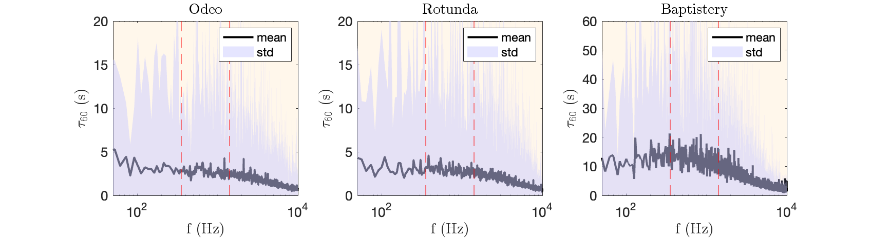
\[ \lambda_i := -\sigma_i + j\sqrt{\Omega_i^2 - \sigma_i^2}, \quad \sigma_i := \frac{3\log(10)}{\tau_{60}}. \]

Modal Shape Recovery via Pole–Residue Least-Squares Fitting

Given poles \( \{\lambda_i\} \), determine residues \( r_i \) from the pole–residue form:

\[ H(j\omega) = \sum_{i=1}^M \left(\frac{r_i}{j\omega - \lambda_i} + \frac{r_i^*}{j\omega - \lambda_i^*}\right), \]

which is linear in \( r_i \). Estimate via least-squares against FRF samples.

Time-Domain Resynthesis

The modal coordinate \( q_i(t) \) satisfies:

\[ \ddot q_i + 2\sigma_i \dot q_i + \Omega_i^2 q_i = c_i f(t) + d_i \dot f(t), \]

with:

\[ \begin{aligned} c_i &= 2\sigma_i \operatorname{Re}(r_i) - 2\sqrt{\Omega_i^2 - \sigma_i^2} \operatorname{Im}(r_i), \\ d_i &= 2\operatorname{Re}(r_i). \end{aligned} \]

Using time step \( T_s \), a stable finite-difference scheme is:

\[ \begin{aligned} q_i^{n+1} = &\; 2q_i^n\cos\left(\sqrt{\Omega_i^2 - \sigma_i^2}\,T_s\right)e^{-\sigma T_s} \\ &- e^{-2\sigma T_s} q_i^{n-1} \\ &+ T_s e^{-\sigma T_s} \left( T_s c_i f^n + d_i(f^n - f^{n-1}) \right), \end{aligned} \]

Finally, the total response is:

\[ y^n = \sum_{i=1}^M q_i^n. \]

Results

Audio Examples

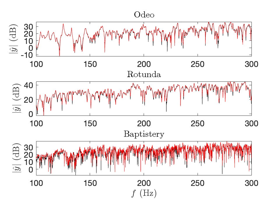
Examples below demonstrate the effect of modal smoothing. Each hall is shown with: (1) measured target RIR, (2) identified response with decay averaging and residue refinement.

Hall	Target RIR	Identified
Odeo Cornaro (Padua)
Rotunda (Bologna)
Baptistery (Pisa)

More Audio Examples

Below are further case studies not described in the paper.

Space	Target RIR	Identified
Example room 1
Example room 2
Example room 3
Example room 4
Example room 5
Example room 6
Example room 7
Example room 8
Example room 9